Triangulation
Introduction
x, y and trivtx
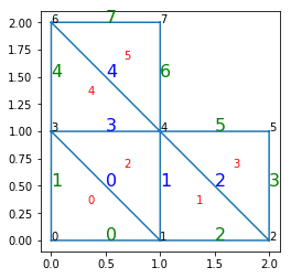
A triangulation is a subdivision of a two-dimensional domain into triangles, defined by:
- its vertices: two 1D arrays
xandyfor coordiantes,- its triangles: one 2D array
trivtx, giving the 3 vertice indices of each triangle.
In [2]:
x = array([0, 1, 2, 0, 1, 2, 0, 1], dtype='d')
y = array([0, 0, 0, 1, 1, 1, 2, 2], dtype='d')
trivtx = array([[0, 1, 3], [1, 2, 4], [1, 4, 3], [2, 5, 4],
                [3, 4, 6], [4, 7, 6]], dtype='int32')

def plot_with_indices():
    # Plot triangulation.
    triplot(x, y, trivtx)

    # Plot vertices indices.
    for ivert, (xvert, yvert) in enumerate(zip(x, y)):
        text(xvert, yvert, ivert)

    # Plot triangle indices.
    for itri, (v0, v1, v2) in enumerate(trivtx):
        xcenter = (x[v0] + x[v1] + x[v2]) / 3.
        ycenter = (y[v0] + y[v1] + y[v2]) / 3.
        text(xcenter, ycenter, itri, color='red')

    axis('scaled')
    show()

plot_with_indices()
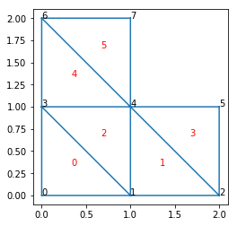
For example, the vertice indices of triangle 2 are:
In [3]:
print(trivtx[2])
[1 4 3]
ga.Triangulation2D
The main purpose of the Triangulation2D
Python extension type is to group this arrays together.
In [4]:
TG = ga.Triangulation2D(x, y, trivtx)
Note
Point2D, Segment2D Triangle2D, etc, are objects that exist in a large number in a program. For example, a numerical simulation may create 10 millions of points. These points will be stored in SoA x and y. There is a Point2D extension type, and an associated CPoint2D C structure that can be stack-allocated for high performance computing on these million of points.
For Triangulation2D, there is typically one or two objects in a program. There do not need stack allocation, and as a such there is no need for C structure.
Iterating on triangle
To iterate a triangle, one first need toextract triangle
vertice indices from trivtx, then vertice coordinates
from x and y.
-
Triangulation2D.get(Triangulation2D self, int triangle_index, CTriangle2D* triangle)
The Triangulation2D.get() method make it a lot easier.
It take as argument the triangle iteration index, and a
c:type:CTriangle2D setted with tree c:type:CPoint2D.
In [5]:
%%cython

from libc.stdio cimport printf
cimport geomalgo as ga

def iter_triangles(ga.Triangulation2D TG):
    cdef:
        int T
        ga.CTriangle2D ABC
        ga.CPoint2D A, B, C

    ga.triangle2d_set(&ABC, &A, &B, &C)

    for T in range(TG.NT):
        TG.get(T, &ABC)
        printf("%d: A(%.0f,%.0f), B(%.0f,%.0f), C(%.0f,%.0f)\n",
               T, A.x, A.y, B.x, B.y, C.x, C.y)
In [6]:
iter_triangles(TG)
0: A(0,0), B(1,0), C(0,1)
1: A(1,0), B(2,0), C(1,1)
2: A(1,0), B(1,1), C(0,1)
3: A(2,0), B(2,1), C(1,1)
4: A(0,1), B(1,1), C(0,2)
5: A(1,1), B(1,2), C(0,2)
-
Triangulation2D.__getitem__(self, triangle_index: int)¶ Return a Triangle2D instance
Computational functions
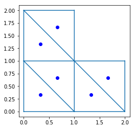
Triangle centers
In [7]:
triplot(x, y, trivtx)

xcenter, ycenter = ga.triangulation.compute_centers(TG)

plot(xcenter, ycenter, 'bo')

axis('scaled')
show()
bounding box
edge lengths
area
Note
Triangulation2D extension type is voluntary keept minimial with 3 attributes and no methods, like above ones could be. The rational behind this is to not impose the application that geomalgo a particular structure, but to let it keep is own: triangular mesh, dual mesh... geomalgo goal is to provide some useful but non-intruise computational primitives.
Boundary and intern edges
A lot of operation on triangulation, for example building a dual mesh, or refining the mesh can be made simple by dealing with boundary edges and intern edges.
-
build_edges(trivtx, NV, intern_edges_order=None, boundary_edges_order=None)¶ Parameters: - It returns:
- a BoundaryEdges object a InternEdges object a EdgeMap object
Boundary edges belongs to 1 triangle, while intern edges belongs
to 2 triangles. Their are build with the build_edges().
In [8]:
intern_edges, boundary_edges, edge_map = ga.build_edges(TG.trivtx, TG.NV)
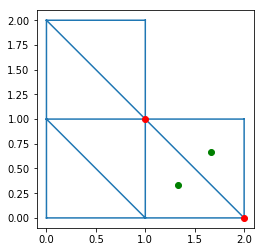
InternEdges has vertices and triangles attributes,
giving the 2 vertices indices and the 2 triangle indices
for each intern edge. For example:
In [9]:
triplot(x, y, trivtx)
I = 2

IA = intern_edges.vertices[I, 0]
IB = intern_edges.vertices[I, 1]
plot([x[IA], x[IB]],
     [y[IA], y[IB]], 'ro')

T0 = intern_edges.triangles[I, 0]
T1 = intern_edges.triangles[I, 1]
plot([xcenter[T0], xcenter[T1]],
     [ycenter[T0], ycenter[T1]], 'go')

axis('scaled')
show()
-
BoundaryEdges.size: int Number of boundary edges in the triangulation.
-
BoundaryEdges.vertices: int[:,:]
-
BoundaryEdges.triangle: int[:]
-
BoundaryEdges.next_boundary_edge: int[:]
-
BoundaryEdges.edge_map: EdgeMap
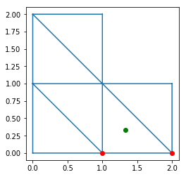
BoundaryEdges has vertices and triangle attributes,
giving the 2 vertices indices and the triangle index
for each boundary edge. For example:
In [10]:
triplot(x, y, trivtx)
I = 2

IA = boundary_edges.vertices[I, 0]
IB = boundary_edges.vertices[I, 1]
plot([x[IA], x[IB]],
     [y[IA], y[IB]], 'ro')

T = boundary_edges.triangle[I]
plot(xcenter[T], ycenter[T], 'go')

axis('scaled')
show()
The third returned object, edge_map, is used to find a intern_edge or boundary_edge given its vertices. It is implemented to be very fast with O(1) complexity.
EdgeMap indexes both InternalEdge and BoundaryEdges. The map_search_edge_idx returns whether the edge is found, and it EdgeMap index. The EdgeMap index is then used to determine whether the edge is a boundary or internal one, and its corresponding index.
In [11]:
%%cython

from libc.stdio cimport printf
cimport geomalgo as ga

def find_edge(ga.EdgeMap edge_map, int IA, int IB):
    cdef:
        bint found
        int E, I

    E = edge_map.search_edge_idx(IA, IB, &found)

    if not found:
        printf("No such edge: (%d,%d)\n", IA, IB)
        return

    I = edge_map.idx[E]

    if edge_map.location[E] == ga.INTERN_EDGE:
        printf("Intern edge for (%d,%d): %d\n", IA, IB, I)
    else:
        printf("Boudnary edge for (%d,%d): %d\n", IA, IB, I)
In [12]:
def text_middle(IA, IB, color):
    A = ga.Point2D(x[IA], y[IA])
    B = ga.Point2D(x[IB], y[IB])
    AB = ga.Segment2D(A, B)
    M = AB.compute_middle()
    text(M.x, M.y, I, color=color, size=16)

for I in range(boundary_edges.size):
    IA, IB = boundary_edges.vertices[I]
    text_middle(IA, IB, 'green')

for I in range(intern_edges.size):
    IA, IB = intern_edges.vertices[I]
    text_middle(IA, IB, 'blue')

plot_with_indices()

find_edge(edge_map, 1, 4)
find_edge(edge_map, 7, 6)
find_edge(edge_map, 7, 5)
Intern edge for (1,4): 1
Boudnary edge for (7,6): 7
No such edge: (7,5)
Locate point
Introduction
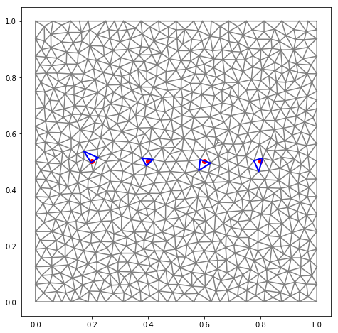
The TriangulationLocator is used to locate in a triangulation
which triangle contains a point.
grid defines the grid size used to speed up the triangle
searching, see Change grid size.
edge_width is used for triange point inclusion tests,
see Triangle2D.include_points().
bounds is an int[NT:4] array allocated to hold temporary value,
an already allocated buffer may be provided.
-
class
TriangulationLocator(self, TG, grid=None, edge_width=-1, bounds=None)¶ Attributes:
-
TG: Triangulation2D
-
grid: Grid2D
-
edge_width: double
-
edge_width_square: double
-
celltri: int[:]
-
celltri_idx: int[:] Cell to triangle map in CSR format.
-
In [13]:
import triangle

def generate_triangulation():
    A = {'vertices' : array([[0,0], [1,0], [1, 1], [0, 1]])}
    B = triangle.triangulate(A, 'qa0.001')
    return ga.Triangulation2D(B['vertices'][:,0],
                              B['vertices'][:,1],
                              B['triangles'])
TG = generate_triangulation()

xpoints = np.array([0.2, 0.4, 0.6, 0.8])
ypoints = np.array([0.5, 0.5, 0.5, 0.5])

locator = ga.TriangulationLocator(TG)
triangles = locator.search_points(xpoints, ypoints)

fig = figure(figsize=(8,8))
ax = fig.add_subplot(1,1,1)
triplot(TG.x, TG.y, TG.trivtx, color='gray')
plot(xpoints, ypoints, 'ro')
for T in triangles:
    TG[T].plot()
axis('scaled')
show()
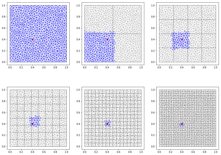
Change grid size
A grid of size \(nx \times ny\) (depending of the number of triangles) is used to map each cells to the triangles it contains. This allow the triangle search performance to be \(O(1)\):
- for a given point, the including cell is found (trivial computation)
- only the triangles in the cells are tested for point inclusion.
The counterpart is the memory usage expanse, as celltri and
celltri_idx grows.
For example:
In [14]:
cell_numbers = array([[1,  2,  4], [8, 16, 32]])

nrows = cell_numbers.shape[0]
ncols = cell_numbers.shape[1]
fig, axes = subplots(ncols=3, nrows=2, figsize=(16,12))

for irow in range(nrows):
    for icol in range(ncols):
        n = cell_numbers[irow, icol]
        fig.sca(axes[irow, icol])

        triplot(TG.x, TG.y, TG.trivtx, color='gray', lw=0.5)

        grid = ga.triangulation.build_grid(TG, nx=n, ny=n)
        grid.plot(color='black', lw=0.5)
        locator = ga.TriangulationLocator(TG, grid)

        P = ga.Point2D(0.4, 0.4)
        P.plot(color='red')

        cell = locator.grid.find_cell(P)

        for T in locator.cell_to_triangles(cell.ix, cell.iy):
            TG[T].plot(lw=0.5)

        print("nx, ny = {}, celltri size: {}, celltri_idx size: {}".format(
                  n, len(locator.celltri), len(locator.celltri_idx)))

        axis('scaled')
show()
nx, ny = 1, celltri size: 1539, celltri_idx size: 2
nx, ny = 2, celltri size: 1679, celltri_idx size: 5
nx, ny = 4, celltri size: 1945, celltri_idx size: 17
nx, ny = 8, celltri size: 2513, celltri_idx size: 65
nx, ny = 16, celltri size: 3909, celltri_idx size: 257
nx, ny = 32, celltri size: 7549, celltri_idx size: 1025
Interpolator
TriangulationInterpolator interpolates data defined on vertices
of a triangulation to given points. NP is the number of points to interpolate
to. gradx, grady and det are double[NT, 3] arrays, computed
with interpolation.compute_interpolator(), which will be invoked if
one the three value is None.
-
class
TriangulationInterpolator(self, TG, locator, NP, gradx=None, grady=None, det=None)¶ Attributes:
-
locator: TriangulationLocator
-
TG: Triangulation2D
-
NP: int
-
gradx: double[NT, 3]
-
grady: double[NT, 3]
-
det: double[NT, 3]
-
triangles: int[NP]
-
factors: double[NT, 3]
-
Points positions are with with TriangulationInterpolator.set_points()
which take a inputs xpoints and ypoints, two double[NP] arrays, and
returns the number of points find out of the triangulation.
-
TriangulationInterpolator.set_points(self, xpoints, ypoints)
Once the points are set, TriangulationInterpolator.interpolate() is called
to interpolate vertdata (double[NV]) to pointdata (``double[NP]). Of course,
it can be called many times of different verdata values.
-
TriangulationInterpolator.interpolate(self, vertdata, pointdata)
In [15]:
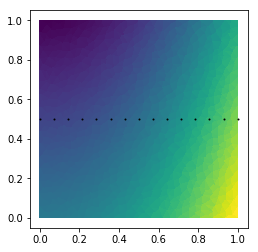
def f(x,y):
    x, y  = np.asarray(x), np.asarray(y)
    return 3*x**2 - 2*y + 2


def g(x,y):
    x, y  = np.asarray(x), np.asarray(y)
    return -x**2 + 0.5*y


# Plot data.
vertdata = f(TG.x, TG.y)
tripcolor(TG.x, TG.y, TG.trivtx, vertdata)
axis('scaled')

# Plot points to interpolate on.
NP = 15
xline = linspace(0, 1, NP)
yline = full(NP, fill_value=0.5)
plot(xline, yline, 'ko', ms=1)
Out[15]:
[<matplotlib.lines.Line2D at 0x7fecc5831f98>]
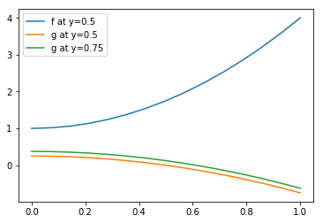
In [17]:
# Interpolate
locator = ga.TriangulationLocator(TG)
interpolator = ga.TriangulationInterpolator(TG, locator, NP)
interpolator.set_points(xline, yline)
linedata = np.empty(NP)
interpolator.interpolate(vertdata, linedata)

# Plot interpolation
plot(xline, linedata, label='f at y=0.5')

# Interpolate other data at the same points
vertdata = g(TG.x, TG.y)
interpolator.interpolate(vertdata, linedata)
plot(xline, linedata, label='g at y=0.5')

# Change points, and reinterpolate
yline[:] = 0.75
interpolator.set_points(xline, yline)
interpolator.interpolate(vertdata, linedata)
plot(xline, linedata, label='g at y=0.75')

legend()
Out[17]:
<matplotlib.legend.Legend at 0x7fecc6155748>
Note
Changing points position imply re-locating triangle and re-computing interpolation factors.
Note
The example interpolate on a line, but there no assumption about it. Points can be unstructured, on a circle, on a cartesian grid, etc.